Molecular docking is often presented with a touch of magic. However, having spent some time in my undergraduate thesis on protein-ligand interactions, I’ve found this perception to be largely misleading. While docking is undeniably a fascinating technique, the reality of docking is much more nuanced.

Traditional experimental techniques such as isothermal titration calorimetry (ITC) or surface plasmon resonance (SPR) can reliably measure binding affinity in-lab, but they’re relatively slow and expensive. Docking allows you to screen thousands if not millions of potential leads in silico before you ever step into a lab.

Yet, it’s not a magic bullet. It’s a fantastic tool, but it also operates on a foundation of assumptions and requires careful preparation to yield meaningful results. It serves as a crude estimator, incredibly useful as long as you know what you’re doing.

This series aims to explore the process over three focused parts:

Part 1: The fundamentals of how molecules bind.
Part 2: A look under the hood at how docking works.
Part 3: A practical guide to doing it right.

This series is intended for anyone with some background in molecular biology and biochemistry. Some of the topics that I will assume you’re familiar with are: protein expression, molecular cloning, and some basic on chemical bond interactions and protein structure. Whether you’re a curious newcomer or you’ve already run a few simulations, I promise there will be something interesting here for you.

Unless otherwise stated, this article will mostly refer to established textbooks and papers as noted in the references [1][2][3][4][5] or considered as general knowledge in the field.

Introduction

Before we simulate any docking experiments, two things must be in place: a solid protein structure and a good understanding of what “binding” actually means physically. First we walk through X-ray crystallography from crystal to PDB entry, highlighting the quality metrics, ranging from resolution, B-factors, R-factor, steric clashes, to Ramachandran plot, occupancy, and more.

We then will explore the thermodynamics of binding, translating the experimental $\Delta G$ into the same force-field components that docking programs estimate: van der Waals interactions, Coulombic interactions, desolvation penalties and the entropy lost upon locking flexible groups. Seeing how these terms actually contribute to the binding energy will let you better judge docking poses and scores.

Proteins and the magic of determining their structure

Proteins are the workhorses of biology, acting as enzymes, receptors, transporters, and structural components that execute various cellular functions. Many of us probably have seen the illustration of a protein 3D structure somewhere. But, have you ever thought, how can we know their structure?

There are many ways we can determine the structure of a given protein, such as x-ray crystallography, nuclear magnetic resonance (NMR), and recently, cryo-EM. As the oldest method amongst the three, x-ray crystallography is the dominant method for determining protein structures. It has tons of drawbacks, sure, but it’s the most established method. X-ray crystallography has been the mainstay historically and still represents the majority of PDB entries, though cryo-EM’s share has grown rapidly for large assemblies[6]. As such, we will talk more about it and put aside the other two methods.

It may be tempting to dismiss this section as too theoretical, after all, we can just download the structure from RCSB. However, the goal of this section is not to teach you on how to do it, but to show the assumptions, limitations, and shortcuts that were made to even have proteins structure. We are not talking about docking yet, the structure determination itself is full of flaws. Every structure, every entry on PDB will have some flaw, either by the experiment or the crystallographer. After all, they’re models, a projection of reality. By knowing those, you can be more skeptical and better manage your expectations on docking results later.

Please note that the majority of things discussed in this section will be about structures determined with X-ray crystallography. Other methods such as Cryo-EM and NMR have different methods, challenges, limitations, metrics, and validation strategies.

X-ray crystallography crash course

Displayed below is the general workflow of x-ray crystallography (see Figure 1). It seems straightforward at first glance: crystallize the protein, shoot it with X-rays, and solve the structure. While the physics and computation can be complex, the biological part seems simple enough. However, you can’t be more wrong. I will explain briefly some of the major challenges of expressing and crystallising the protein, then the complexity of the modelling and refining the model afterwards.

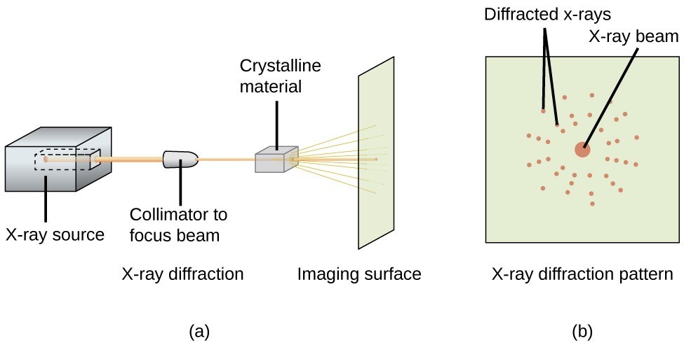
General workflow of x-ray crystallography.

Figure 1: General workflow of x-ray crystallography.
[By Jonathan Gutow, CC BY 4.0, Chem Libretext]

The struggle of crystallisation

Before we can even begin, we need to produce a large quantities of pure and stable samples of our protein of interest. Most proteins are simply not abundant enough in their native sources, hence we often resort to heterologous expression, that is expressing a protein outside of its native organism; most frequently one of the many designd E. coli strains like BL21, yeasts, or even mammalian expression system such as Human Embryonic Kidney (HEK). This is where the problem begins.

Different organisms have different cellular internal environments and molecular machinery. For example, different organisms have different codon preferences, hence we need to optimize the codons for our genetic code. Thankfully, modern bioinformatics has made this hardly a problem since codon optimizers are widely available.

A more pressing issue is that of post-translational modifications (PTMs). Prokaryotes generally lack PTMs, unlike eukaryotes. While the absence of PTMs can be an advantage, as we can avoid the problem of conformationally heterogeneous glycosylation, the lack of PTMs can still render the protein nonfunctional. However, if the protein’s fold is not compromised, the structure can still provide insights, albeit with caveats. Secondly, protein expression induces metabolic stress in the host. If not handled properly, this can cause misfolding, resulting in inclusion bodies. Heterologous organisms also don’t always have the necessary chaperones to fold the protein correctly. Last but not least, disulfide bonds (Cys-S-S-Cys) require the chemical oxidation of two adjacent cysteines to form. Unfortunately, a bacterium’s intracellular environment is generally reducing, which means complex disulfide bond formation in the cytoplasm sometimes fails to occur properly. This problem can be alleviated by using yeast or other eukaryotic expression systems, but specialized E. coli strains that have mutations in the trxB and gor genes can also be used.

We won’t talk too much about fusions and tags since they’re beyond the scope of this post, but you need to remember that these are also needed for purification, adding another factor to our already complex situation.

Next, crystallisation. What is a crystal anyway? Crystals are basically just an array of highly ordered molecules. Table salt is a common example of crystal. However, unlike table salt (NaCl) which has a strong bond thanks to their strong ionic bond, proteins don’t get to enjoy that kind of luxury. Protein crystals are largely kept together by weaker forces between side-chains, such as vdW, hydrogen bond, and so on. As for the crystallisation process itself, basically we tries to nudge the proteins to a state of supersaturation by slowly removing solvents. However, that process, more often than not, fails miserably. We need to repeat our experiments multiple times, using different solvents, additives, concentration, pH, temperature, and so on until it’s just right for the proteins to crystallise (most commonly using vapor diffusion methods like hanging drop). Some proteins can’t even be crystallised, at all. Some suggests that the reason why proteins don’t crystallise well is perhaps due to evolutionary reason: you don’t want your proteins to clump together in the nature.

Salt crystals (NaCl)

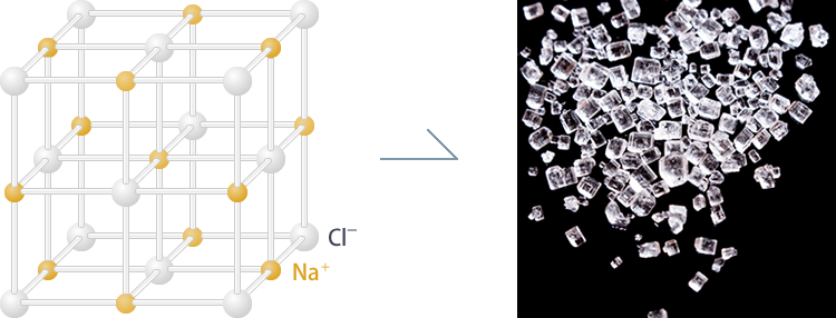
Figure 2: Salt crystals (NaCl).
[By Japan Aerospace Exploration Agency (JAXA), © JAXA, Humans in Space]

Protein crystals (haemoglobin)

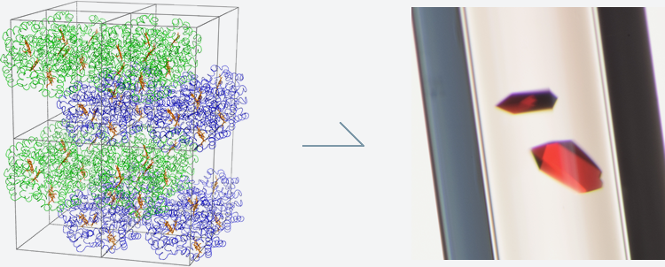
Figure 3: Protein crystals (haemoglobin).
[By Japan Aerospace Exploration Agency (JAXA), © JAXA, Humans in Space]

A good crystal should be well ordered with minimal deformities, otherwise the resulting diffraction pattern can be poor and unusable for downstream processing. Hence, merely having a crystal is not enough. Methods such as Surface Entropy Reduction (SER) is sometimes used to reduce entropy on the surface. The idea is to identify surface residues with long, flexible side chains, such as lysine and to replace them with small, more rigid residue, such as alanine. By mutating those floppy surface side chains, the entropic penalty for crystallisation can be minimised, making the process easier to achieve. One might ask: “Wont that change the conformation?” Well, yeah, but we can try to use computational model to minimise the potential effect, especially near critical regions like binding site. After all, even the crystallisation process itself can introduce problems like crystal packing artifacts.

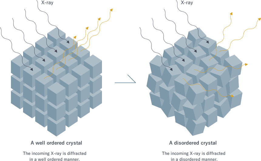
Illustration of well ordered crystal.

Figure 4: Illustration of well ordered crystal.
[By Japan Aerospace Exploration Agency (JAXA), © JAXA, Humans in Space]

To illustrate how crystallisation can introduce problems, consider the case of HIV-1 integrase. In its first crystal structure (PDB: 1itg), the protein was crystallised in the presence of cacodylate [7]. That cacodylate happened to attach itself covalently to a cysteine in the enzyme’s active site. Because of this attachment, the key catalytic residues: Asp64, Asp116, and Glu152, ended up arranged in the wrong geometry [8][9]. The structure looks valid crystallographically, but it wasn’t biologically accurate since it made the enzyme looked inactive. It only became clear that the catalytic residues had been “knocked out of alignment” when later structures from HIV-1 integrase crystals grown without cacodylate were solved. In those, the enzyme appeared in its proper functional geometry [10][11].

Lysozyme crystals observed through polarizing filter in Nikon SMZ800 microscope.

Figure 5: Lysozyme crystals observed through polarizing filter in Nikon SMZ800 microscope.
[By Taavi Ivan, CC BY-SA 3.0, Protein Diffraction]

If somehow, by divine benevolence, you manage to crystallise your protein of interest, you will get pretty looking crystals, like the one displayed in Figure 5. One interesting property of protein crystals are that they behave different optically, hence we can use polarising lens to differentiate our crystal from salt crystals. Once we have our crystals prepared, we can do the diffraction experiment by shining x-rays to our crystals, and recording the diffraction pattern.

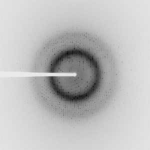
$Example of a diffraction data (PDB ID: 4W65).$

Figure 6: Example of a diffraction data (PDB ID: 4W65).
[Seattle Structural Genomics Center for Infectious Disease (SSGCID), Davies, D.R., Dranow, D.M., Lorimer, D., Edwards, T.E., CC0, Protein Diffraction]

Illustration of the electron density map of 6GLP, visualised with COOT.

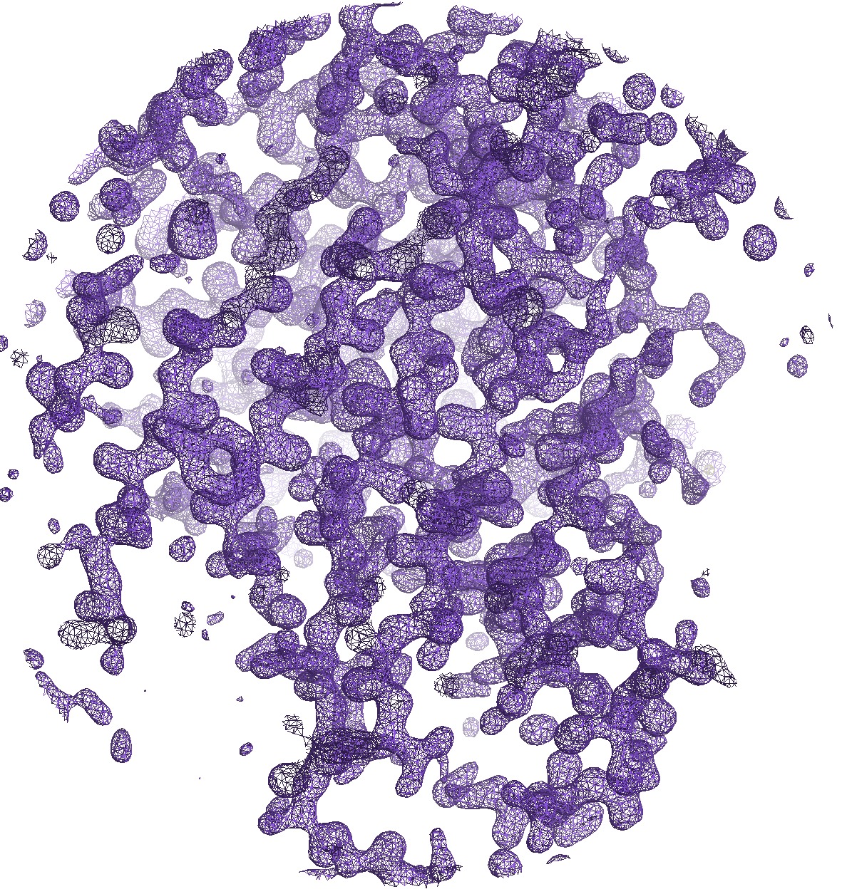
Figure 7: Illustration of the electron density map of 6GLP, visualised with COOT.
[By Rayhan M, CC BY 4.0]

Having done our diffraction experiment, the result is a bunch of intensity data. However, intensity alone is not enough to perform an inverse Fourier transform. We need to know the phase too. To know more about it, open the toggle about phase problem below. Once we have our phase, we now have an electron density map. Basically, we can “see” how the electrons of our protein is mapped in 3D space. So, we don’t directly get the residues or even the atoms, only the distribution of the electrons. One such example can be seen on Figure 7 as visualised with COOT. Afterwards, the job of deciding what residue belongs to each site falls upon the crystallographer. They’re tasked with “guessing” which residue is producing said electron density map. Of course, it’s not totally random, we can make educated guesses by the shape and length of the blob. For example, in Figure 10, we can guess that it’s a Tyr since it has a visible shape of a phenol ring. For proteins that have been solved before or have similar homology, we can also use molecular replacement to get the initial model.

Phase Problem in X-ray Crystallography

▼

Here’s where things get tricky. When X-rays scatter off our protein crystal, we can measure the intensity of the diffracted beams, but we lose crucial information about their phase. Think of it like this: imagine you’re trying to reconstruct a complex wave pattern, but you can only see how bright each point is, not whether the wave is going up or down at that moment. At the time of writing, we don’t have any good instrument to measure oscillations at such rapid rate either.

In mathematical terms, each diffracted beam can be described as a complex number with two components: amplitude ( $|F|$ ) and phase ( $\phi$ ). The structure factor can be described as $F(hkl)$ = $|F|e^{i\phi}$ , where hkl are the Miller indices describing the diffraction spot. Recall that we can determine the structure factors of our by the electron density distribution within the crystal unit cell using the forward Fourier transform.

F(hkl) = \int_{V} \rho(xyz) e^{2\pi i (hx+ky+lz)} dV

$F(hkl)$ is the structure factor for a given diffraction spot with Miller indices $hkl$ . It’s a complex number containing both the amplitude (which we measure as the intensity) and the phase (which is lost). $\rho(xyz)$ is the electron density at a fractional coordinaate $(x,y,z)$ which is what we want as our electron density map, $V$ represents the volume of the unit cell, and $e^{2\pi i (hx+ky+lz)}$ is the phase factor that describes how a wave scattered from a point $(x,y,z)$ contributes to the overall diffraction beam in the $(h,k,l)$ direction.

Interestingly, we can invert the equation to get the electron density distribution from the structure factors, described as follows:

\rho(xyz) = \frac{1}{V} \sum_{h} \sum_{k} \sum_{l} F(hkl) e^{-2\pi i (hx+ky+lz)}

However, to reconstruct the electron density map using the inverse Fourier transform above, we need both the amplitude and the phase of every diffracted beam, since $F(hkl) = |F|e^{i\phi}$ . Without the phase information, we’re essentially trying to solve a puzzle with half the pieces missing. One classic example of this can be seen on Figure 8. We perform Fourier transform to both the image of a cat and a duck, then do the inverse Fourier transform with the phase swapped. As you can see, the resulting image follows the phase of the original image more (e.g., cat amplitude with duck phase resembles a duck, vice versa). So, clearly phase resembles the bulk of informations.

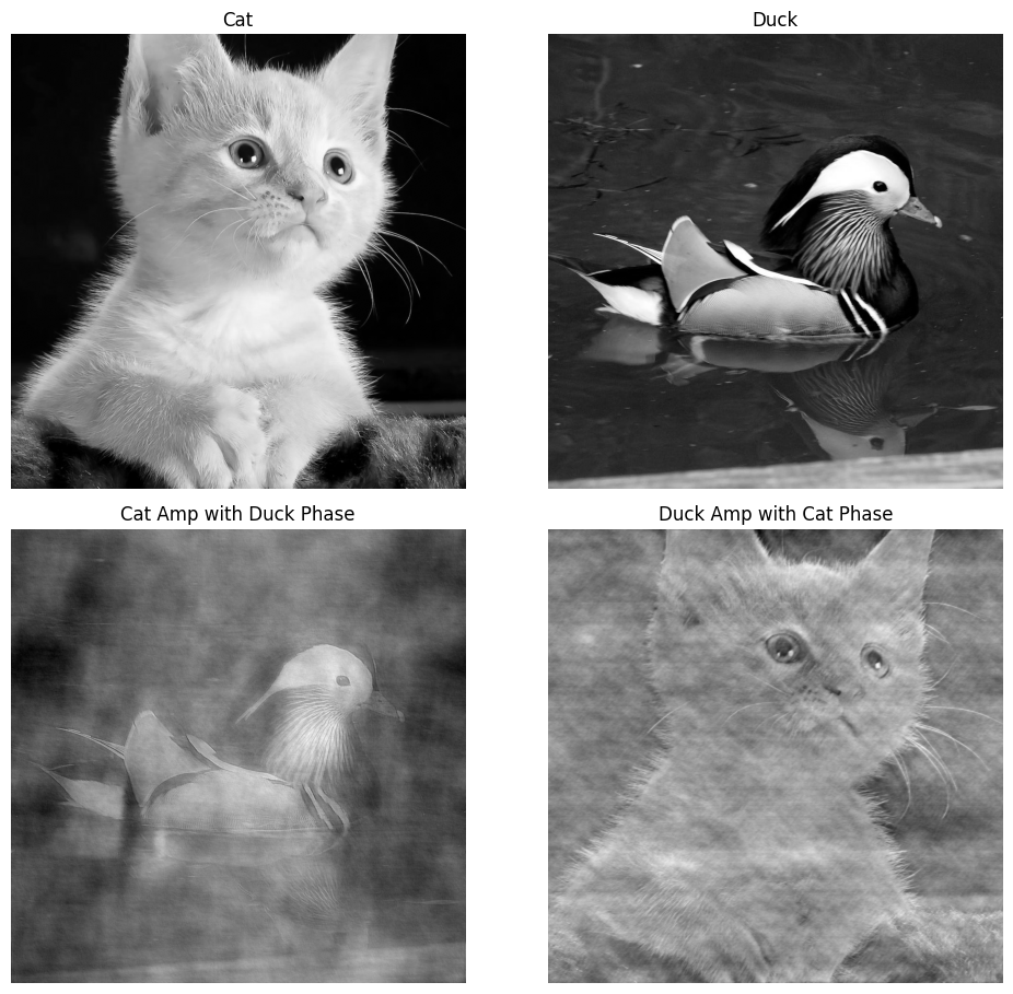
Phase problem illustration with both amplitude and phase information.

Figure 8: Phase problem illustration with both amplitude and phase information.
[By Rayhan M, CC BY 4.0]

However, if we only have the amplitude information, the resulting image is essentially meaningless noise, as can be seen on Figure 9. Hence, we need to somehow get the phase information.

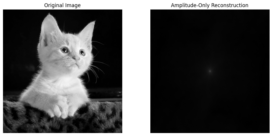
Phase problem illustration with amplitude information only.

Figure 9: Phase problem illustration with amplitude information only.
[By Rayhan M, CC BY 4.0]

To overcome this, crystallographers developed several ingenious strategies. The classic approach involves using heavy atoms, a method known as multiple isomorphous replacement (MIR). The idea is to soak the protein crystal in a solution containing heavy atoms, like mercury or gold. These atoms are so electron-dense that they dramatically alter the diffraction pattern. By comparing the data from a native crystal to one with heavy atoms, you can pinpoint the locations of those few heavy atoms. Their positions then provide a rough estimate of the phases for the entire structure, which you can refine further afterward.

Today, the most common technique is molecular replacement (MR), which you can use if there is previously solved structure of a similar protein. It calculates a theoretical diffraction pattern at each position and compares it to your experimental data. The orientation that produces the best match is declared the winner, and the phases from that correctly placed model are used as an excellent starting point. For those familiar with in silico protein structure determination, this technique is akin to homology modelling used by SWISS-MODEL. It’s important to note that MR can introduce model bias, which is a problem in itself.

Another modern method is anomalous scattering like single-wavelength anomalous diffraction (SAD). This technique exploits a quirk of physics where, if you tune your X-ray beam to a very specific wavelength (right near the “absorption edge” of an atom in your crystal), that atom scatters the X-rays differently. This subtle effect breaks a rule called Friedel’s Law, creating small but measurable differences between reflections that would otherwise be identical. These tiny differences are directly related to the phase, allowing you to calculate the phases from scratch. However, anomalous scattering techniques usually requires synchotron, which is not always available on many labs. Still, this technique is promising because it only requires single type of crystal unlike MIR and can work for novel structures.

Finally, for small molecules, crystallographers can often use direct methods which uses pure mathematical approach that relies on the fact that electron density is always positive and concentrated in atom-sized lumps. These constraints create statistical relationships between the phases of the strongest reflections. For a small molecule, algorithms can use these relationships to test different phase combinations and directly converge on the correct solution. However, for large proteins, the number of possibilities becomes too vast to solve.

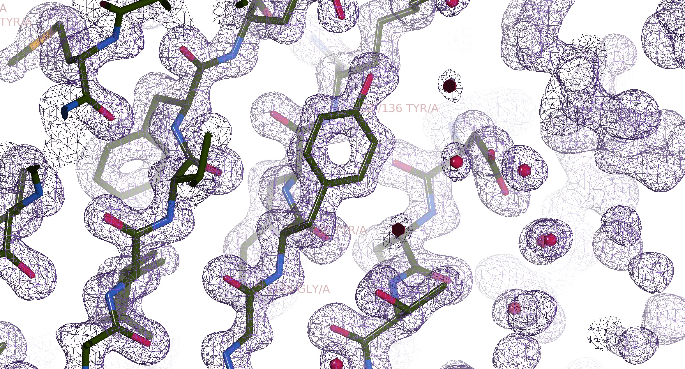
Illustration of the electron density map of 6GLP, visualised with COOT.

Figure 10: Illustration of the electron density map of 6GLP, visualised with COOT.
[By Rayhan M, CC BY 4.0]

Since we are modelling based on the electron density map, the resolution of the EDM matters a lot. To see why, let’s take a look at Figure 11. As the resolution worsens from 1.0 to 6.0 $\AA$ , we can see that the EDM gets more and more fuzzy, and the detail of the structure gets lost. We may still be able to see the general shape of the protein, but the details are lost. This is why we care about the resolution of the EDM, because low resolution EDM forces us to make more assumptions regarding the exact positions of the atoms.

Figure 11: EDM comparison of various resolutions from 1.0 to 6.0 $\AA$ , visualised with ChimeraX. The EDM is generated from the model, hence it doesn’t have noises that exist in real experimental EDM.
[By Rayhan M, CC BY 4.0]

It’s also important to note that most protein structure data don’t include hydrogen atoms, due to their size. Remember that hydrogen only has 1 electron, as opposed to other atoms such as carbon, which has 6 electrons, or oxygen, which has 8 electrons. Therefore, the electron density of hydrogen is very low, making it hard to resolve with X-ray crystallography. Sub-angstrom resolution has been achieved with various techniques, hence allowing us to resolve hydrogen atoms[12], but it’s still relatively rare.

For this reason, we usually need to add hydrogen atoms to our model explicitly, often called protonation. Protonation is a tricky process. There are a lot of nuances that can break your model. For example, histidine is famous for its pKa of 6.0, which is very close to physiological pH. Because of this proximity, small fluctuations in the local pH can shift the equilibrium of its side chain (an imidazole ring). It has two tautomers at neutral condition, called HIE where the proton is on the epsilon nitrogen and HID where the proton is on the delta nitrogen. When both are protonated, histidine will be positively charge, called HIP. You can’t just ignore histidine as they’re very important for biological processes. They’re famous as a master of catalyst by acting as a proton shuttle. They’re also good as a metal coordinator, like in hemoglobin. As such, we can’t just blindly add hydrogens to our model, more elaborate tools like PROPKA[13][14] might be needed to handle His properly.

Assessing model quality

Validating and assessing model quality should be done hand-in-hand with the modelling and refinement process. However, as a user, you still need to know how to assess the quality of the model you’re using after they’re being deposited. Hence, we will talk about some of the important metrics you can use for that.

Resolution

Crystallographic resolution is an important measure of the quality and detail in a structure determined by X-ray diffraction. At its core, resolution in crystallography is a measure of the smallest distance at which two individual features can be distinguished in the calculated electron density map. A “high-resolution” structure, indicated by a low value (e.g., 1.5 $\AA$ ), means that the atomic positions are well-defined and individual atoms can be clearly observed. Conversely, a “low-resolution” structure, represented by a higher value (e.g., 3.5 $\AA$ ), will only show the general outline of the molecular backbone.

However, resolution is not a great metric to solely rely on. It’s a global-metric and resolution is not homogenous throughout the whole structure. There are other factors that can affect resolution, such as B-factor and occupancy. Hence, we should treat this metric with a grain of salt and instead take a deeper look into your structure of interest.

Resolution Limits and Electron Density Peaks

▼

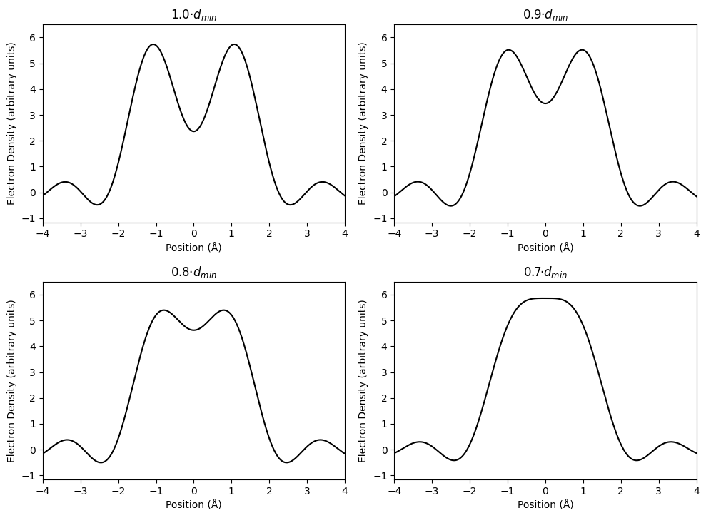
Electron density peak resolution, plot inspired by Benhard Rupp (Biomolecular Crystallography 2010 pp. 453)

Figure 12: Electron density peak resolution, plot inspired by Benhard Rupp (Biomolecular Crystallography 2010 pp. 453).
[By Rayhan M, CC BY 4.0]

One common misconception is that the resolution stated in crystallographic table ( $d_{min}$ ) represents the limit of resolution (LoR). However, that is only a conservative approximation. An analysis by R.E. Stenkamp and L. H. Jensen showed that for the kind of reconstruction done for X-ray crystallography, the LoR is $0.917 \cdot d_{min}$ . We have established before that LoR is affected by B-factor, but this limit works reasonably well even for B-factors up to 10 $\AA^2$ . In Figure 12, we can see that for a unit cell of 20 $\AA$ , two oxygen atoms with full occupancy, B-factor of 10 $\AA^2$ , with varying distance of 1.0, 0.9, 0.8, and 0.7. We can still reasonably differentiate the peak of the two atoms at $0.9 \cdot d_{min}$ , dubious at $0.8 \cdot d_{min}$ , and impossible at $0.7 \cdot d_{min}$ .

B-factor

Figure 13: Visualization of B-factors in a protein structure (PDB ID: 2B3P). Red regions indicate high B-factors, blue regions show low B-factors, visualised with ChimeraX.
[By Rayhan M, CC BY 4.0]

B-factor is a value assigned to each atom in the crystal structure that quantifies its degree of thermal motion or static disorder. In simpler terms, it measures how much an atom “wobbles” or deviates from its average position within the crystal lattice. A low B-factor means an atom is well-ordered and its position is precisely defined in the EDM. Modelling B-factor allows us to make our model calculated EDM closer to the experimental data, which makes crystallographer happy. These are typically atoms in the core of a protein. In contrast, a high B-factor indicates that an atom is more mobile or exists in multiple conformations, which is common for flexible loops.

Regions of a protein with high B-factors inherently correspond to areas of lower local resolution. In these flexible regions, the electron density is smeared out, making the precise placement of atoms more ambiguous. Conversely, parts of the structure with low B-factors are well-ordered and contribute to the high-resolution features of the electron density map. Therefore, while a single resolution value is often assigned to an entire structure, the B-factors reveal the underlying heterogeneity. Moreover, if an atom wobbles too much, a crystallographer might even mark the atom or even the whole residue as missing, which you should fix before docking. To better illustrate how local resolution can differ, consider the picture below in Figure 14. Some objects in the photo are sharp, while others are blurry due to their movement when the photo is taken. The sharpness of the object is analogous to the local resolution of the atom. If your binding pocket has a high B-factor, that means the structure there is not well-resolved, and you might need to interpret your docking result with a grain of salt.

Edited phi dihedral angle rotation example

Original phi dihedral angle rotation example

Figure 14: Real life illustration of b-factor, blue indicating low b-factor, while red indicating high b-factor. Slide from A to B to see the difference.
[Original photo by Pew Nguyen, CC BY 4.0, Pexel]

There are two possible causes for this artifact. The first one is called static disorder. Since our diffraction experiment uses protein crystals, which in itself consists of many proteins, some differences are bound to happen. Not every protein will fold in the exact same way. In practice, we usually average them out, by this can cause the electron density map to be “fuzzy” if the conformations vary wildly from unit cells to the others. Think of it like telling a bunch of people to strike a peace pose, it’s bound to have some variance since every person might interpret it differently.

Secondly, there’s this thing called dynamic motion. As we all know, proteins are not static, atoms are not either. Even when being crystallised, some random motions at the atomic level is still bound to happen, particularly among places where they’re not too rigid (e.g., side-chains). Think about this one like capturing people standing still. Even if we assume that they’re able to stand perfectly still, some little movements are still inevitable.

More about B-factor

▼

There are various ways to represent B-factors. Isotropic B-factor is the most common type, which assumes atomic displacement is equal in all directions (spherical symmetry). Due to its simplicity, isotropic b-factor can be easily optimised during refinement process since it only consists of 1 parameter.

However, as you can already guess, atoms don’t move in a perfect sphere of motion. Hence, some people opt to use anisotropic B-factor, which represents atomic displacement with 6 parameters to represent ellipsoidal displacement. Anisotropic B-factor is usually stored in the ANISOU record. While it is a more accurate model, it’s also hard to refine due to the number of parameters involved. It also requires high resolution data for refinement.

To accomodate lower resolution structure data, some use TLS models atomic displacement. TLS is a combination of: Translation (T) which represents rigid body movement; Libration (L) which represents rotational motion around a point; and Screw (S) which represents coupled translational and rotational motion. TLS can work with lower resolution structure and is more efficient since you can model hundreds or even thousands of atoms instead of refining them individually.

For docking, high B-factor regions may need special attention since their position is uncertain. If available, anisotropic B-factors can provide more reliable insight on the atomic positions, while TLS can inform which parts of the protein are likely to move during binding.

Occupancy

Alternative conformation of Arg63 in 2AXW, visualised in RCSB. Highlighted with pink overlay is the side-chain alternative conformation.

Figure 15: Alternative conformation of Arg63 in 2AXW, visualised in RCSB. Highlighted with pink overlay is the side-chain alternative conformation.
[By Rayhan M, CC BY 4.0]

People often confuse between occupancy and B-factor. They’re related, but fundamentally different. Occupancy is the percentage of samples that contain a particular atom. If it’s 1.00, it means the atom is present in all samples. If it’s 0.50, it means the atom is present in half of the samples. This is often seen in the case of side-chain alternative conformations. For example, in Figure 15, Arg63 has two alternative conformations, one is the “normal” one, and the other is the “flipped” one. The “flipped” one is present in half of the samples. Therefore, the occupancy of Arg63 is 0.50 for each conformation.

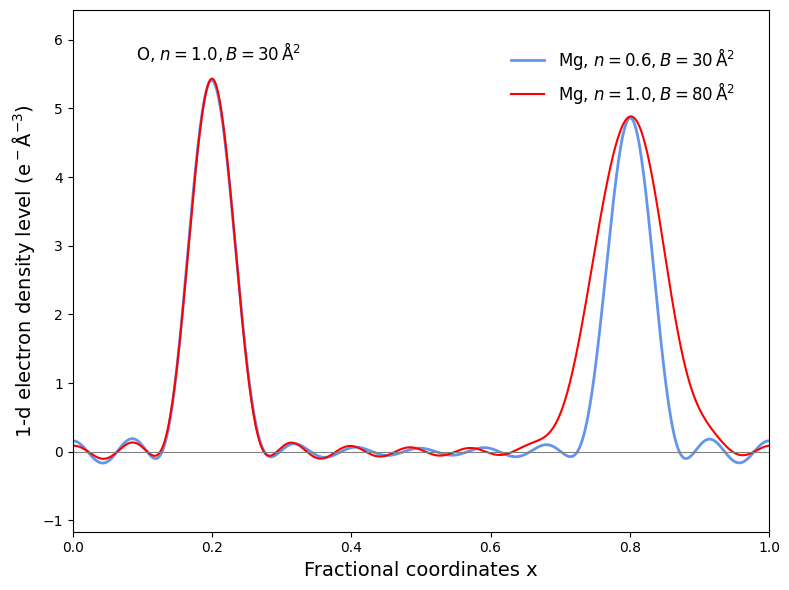
Illustration of the electron density map of 2AXW, visualised with COOT.

Figure 16: Electron density peak of Mg and O with various occupancy and B-factor.
[By Rayhan M, CC BY 4.0]

Unfortunately, the data is not always conclusive enough to support the existence of a different conformation. In this case, the occupancy is 1.00 for all samples, but the crystallographer will assign a high B-factor to the atom to indicate that it’s not well-ordered. For example, if you look at Figure 16, the peak of Mg with a low B-factor but high occupancy is quite similar to the peak of Mg with high B-factor but low occupancy. This is often called as B-factor/occupancy correlation. Moreover, it can also difficult to differentiate heavier and lighter atom if the B-factor is quite high, as shown with the similar peak of O ( $z$ =8) and Mg ( $z$ =12) at a resolution of 1.8 $\AA$ . In real case, we can try to distinguish the two based on bond distances and coordination geometry of the atom, but it’s still tricky nonetheless.

You can see below how the different conformations are represented in the PDB file of 2AXW for Arg63, specifically starting from line 993 (e.g., AARG and BARG).

# Snippet from the PDB file of 2AXW for Arg63
ATOM    989  N   ARG A  63       6.993  48.721  17.381  1.00  7.41           N  
ANISOU  989  N   ARG A  63     1121    819    875    -66      5    -18       N  
ATOM    990  CA  ARG A  63       7.475  47.391  17.007  1.00  7.44           C  
ANISOU  990  CA  ARG A  63     1040    877    910   -124     36     26       C  
ATOM    991  C   ARG A  63       6.307  46.427  16.943  1.00  7.26           C  
ANISOU  991  C   ARG A  63     1010    899    848    -47     80      3       C  
ATOM    992  O   ARG A  63       5.514  46.344  17.887  1.00  7.45           O  
ANISOU  992  O   ARG A  63      984    932    912    -91     49   -112       O  
ATOM    993  CB AARG A  63       8.489  46.932  18.030  0.50  8.16           C  
ANISOU  993  CB AARG A  63      952   1062   1085   -114    -54     68       C  
ATOM    994  CB BARG A  63       8.501  46.882  18.008  0.50  8.71           C  
ANISOU  994  CB BARG A  63     1066   1088   1153    -76    -93     67       C  
ATOM    995  CG AARG A  63       9.361  45.817  17.673  0.50  9.04           C  
ANISOU  995  CG AARG A  63     1173    987   1272    -76    130     41       C  
ATOM    996  CG BARG A  63       9.857  47.509  17.828  0.50 11.24           C  
ANISOU  996  CG BARG A  63     1327   1429   1513   -218   -192     30       C  
ATOM    997  CD AARG A  63      10.169  45.309  18.897  0.50 11.98           C  
ANISOU  997  CD AARG A  63     1297   1687   1568     14   -148    -37       C  
ATOM    998  CD BARG A  63      10.981  46.795  18.527  0.50 14.43           C  
ANISOU  998  CD BARG A  63     1610   1897   1976    -14   -119     24       C  
ATOM    999  NE AARG A  63      11.112  46.323  19.377  0.50 15.40           N  
ANISOU  999  NE AARG A  63     1964   1917   1970    -50    -12   -145       N  
ATOM   1000  NE BARG A  63      11.146  45.427  18.062  0.50 16.21           N  
ANISOU 1000  NE BARG A  63     2214   1949   1994     19    -59    -29       N  
ATOM   1001  CZ AARG A  63      12.437  46.270  19.217  0.50 19.07           C  
ANISOU 1001  CZ AARG A  63     2174   2548   2521    -37     92    -75       C  
ATOM   1002  CZ BARG A  63      12.193  44.636  18.320  0.50 17.96           C  
ANISOU 1002  CZ BARG A  63     2274   2328   2222     43     48     -6       C  
ATOM   1003  NH1AARG A  63      13.018  45.251  18.586  0.50 19.99           N  
ANISOU 1003  NH1AARG A  63     2344   2778   2472     93    178    -49       N  
ATOM   1004  NH1BARG A  63      13.238  45.076  19.010  0.50 20.32           N  
ANISOU 1004  NH1BARG A  63     2432   2800   2486      5      3      6       N  
ATOM   1005  NH2AARG A  63      13.196  47.250  19.700  0.50 18.22           N  
ANISOU 1005  NH2AARG A  63     2123   2360   2439     95    158    -94       N  
ATOM   1006  NH2BARG A  63      12.180  43.389  17.862  0.50 14.68           N  
ANISOU 1006  NH2BARG A  63     1681   2116   1777    323      6    165       N  
ATOM   1007  H   ARG A  63       6.957  48.858  18.222  1.00  7.57           H  
ATOM   1008  HA  ARG A  63       7.904  47.430  16.129  1.00  7.71           H  
ATOM   1009  HB2AARG A  63       9.063  47.688  18.227  0.50  8.06           H  
ATOM   1010  HB2BARG A  63       8.197  47.083  18.907  0.50  8.61           H  
ATOM   1011  HB3AARG A  63       8.012  46.680  18.837  0.50  8.06           H  
ATOM   1012  HB3BARG A  63       8.594  45.922  17.902  0.50  8.61           H  
ATOM   1013  HG2AARG A  63       8.801  45.096  17.356  0.50 10.37           H  
ATOM   1014  HG2BARG A  63      10.070  47.530  16.882  0.50 11.96           H  
ATOM   1015  HG3AARG A  63       9.984  46.109  16.988  0.50 10.37           H  
ATOM   1016  HG3BARG A  63       9.822  48.411  18.174  0.50 11.96           H  
ATOM   1017  HD2AARG A  63       9.554  45.125  19.620  0.50 13.52           H  
ATOM   1018  HD2BARG A  63      11.805  47.277  18.357  0.50 15.23           H  
ATOM   1019  HD3AARG A  63      10.639  44.498  18.659  0.50 13.52           H  
ATOM   1020  HD3BARG A  63      10.799  46.769  19.479  0.50 15.23           H  
ATOM   1021  HE AARG A  63      10.742  47.189  19.592  0.50 17.17           H  
ATOM   1022  HE BARG A  63      10.697  45.242  17.229  0.50 17.89           H  
ATOM   1023 HH11AARG A  63      12.557  44.604  18.264  0.50 21.28           H  
ATOM   1024 HH11BARG A  63      13.255  45.876  19.321  0.50 21.33           H  
ATOM   1025 HH12AARG A  63      13.874  45.239  18.495  0.50 21.28           H  
ATOM   1026 HH12BARG A  63      13.904  44.553  19.159  0.50 21.33           H  
ATOM   1027 HH21AARG A  63      12.837  47.911  20.108  0.50 21.00           H  
ATOM   1028 HH21BARG A  63      11.516  43.092  17.410  0.50 19.41           H  
ATOM   1029 HH22AARG A  63      14.050  47.224  19.601  0.50 21.00           H  
ATOM   1030 HH22BARG A  63      12.850  42.880  18.008  0.50 19.41           H

R-factor

R-factor quantifies how well the refined atomic model agrees with the original experimental diffraction data. It measures the discrepancy between the amplitude calculated from your model ( $|F_{calc}|$ ) and those observed in the experiment ( $|F_{obs}|$ ). It can be described mathematically as:

R = \frac{\sum_{hkl} ||F_{obs}(hkl)| - |F_{calc}(hkl)||}{\sum_{hkl} |F_{obs}(hkl)|}

A lower R-factor indicates a better fit between the model and the data, with zero meaning a perfect match. However, it’s never achieved in practice due to experimental noise and model imperfections. A very low R-factor isn’t always good either; it could mean the model has been overfitted to the noise in the data.

To prevent this, we can use another metric called $R_{free}$ . Before refinement, a small subset of the diffraction data (typically 5-10%) is set aside and not used in the model-building process, hence it serves as an unbiased check. If a model is genuinely accurate, it will not only fit the data it was built with, but also predict the unseen data well. If R-free is significantly higher than R-work (>5%), it suggests that the model might have been overfitted. Some people, have proposed an even tighter metric, called $R_{sleep}$ , which contains data that has never been used at all. However, it’s still rarely used, since adding another holdout set means you will reduce even more data from the dataset.

One interesting thing to note is the R-factor’s relationship with the crystallographic phase problem. The R-factor directly compares amplitudes ( $|F_{obs}|$ vs. $|F_{calc}|$ ), because the experimental data contains no phase information.

However, the phases used in model building ( $\phi_{calc}$ ) are calculated from the coordinates of the atoms in your model. The refinement process works by adjusting these atomic coordinates to make the calculated amplitudes ( $|F_{calc}|$ ) better match the observed ones ( $|F_{obs}|$ ), which is what minimizes the R-factor. Because a single atomic model generates both the calculated amplitudes and phases, the R-factor serves as an indirect measure of your model’s correctness, and by extension, the quality of your phase estimates. A model that is accurate enough to yield a low R-factor is also very likely to be producing reliable phases.

Steric clashes

Another critical quality check is for steric clashes. Think of an atom as having an invisible “personal space” bubble around it. The radius of this bubble is called the van der Waals (vdW) radius. It represents the distance from the atom’s nucleus to the point where the attractive forces with a neighboring, non-bonded atom are perfectly balanced by the strong repulsive forces between their electron clouds.

So, why can’t this boundary be crossed? The answer lies in the Pauli Exclusion Principle from quantum mechanics, which states that no two electrons can occupy the same quantum state. As two atoms get closer than their combined vdW radii, their electron clouds begin to overlap. This forces electrons into higher energy orbitals, creating an incredibly strong repulsive force that pushes the atoms apart. The energy of this repulsion skyrockets as the distance shortens (it’s proportional to $(\frac{1}{r})^{12}$ in the Lennard-Jones potential we’ll discuss later). A steric clash in a model represents this physically impossible overlap. High-quality structures will have very few to no steric clashes. You can check for this metric using tools such as MolProbity and PROCHECK. Usually RCSB will have already done that for you, though, just check their structure summary.

Ramachandran plot

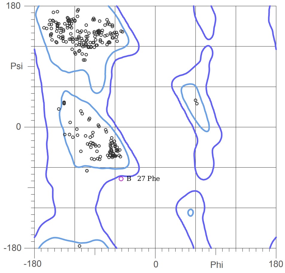
General Ramachandran plot of 6GLP, visualised with MolProbity

Figure 17: Ramachandran plot of 6GLP, visualised with MolProbity.
[By Rayhan M, CC BY 4.0]

Finally, we have the Ramachandran plot. This plot can be used for checking the stereochemical quality of a protein’s backbone. It maps the two main dihedral angles of the polypeptide backbone, phi ( $\phi$ , the C-N-C $\alpha$ -C bond) and psi ( $\Psi$ , the N-C $\alpha$ -C-N bond), for every amino acid. The rotation around these bonds is restricted because of steric hindrance between atoms in the backbone and the side chain. The Ramachandran plot visualizes these sterical combinations.

Psi dihedral angle rotation example in protein backbone.

Figure 18: Psi dihedral angle rotation example in protein backbone.
[By Eric Martz, CC BY-NC-SA 4.0, YouTube]

Phi dihedral angle rotation example in protein backbone.

Figure 19: Phi dihedral angle rotation example in protein backbone.
[By Eric Martz, CC BY-NC-SA 4.0, YouTube]

As illustrated on Figure 18 and Figure 19, as you rotate the psi and phi bond, sometimes you encounter steric clashes, making some angles physically implausible. Based on those angles, we can split the regions in Ramachandran plot into three categories:

Most Favorable Regions: These are areas where the backbone atoms are comfortably far apart. A good structure will have >90-95% of its residues here.
Allowed Regions: Conformations that are less common, but still physically possible.
Disallowed Regions: Conformations where atoms would clash severely. A residue in this region is a major red flag.

Of all the amino acids, Glycine is a major exception because its side chain is just a single hydrogen atom, giving it more rotational freedom. Proline is the opposite with its side chain forming a ring with the backbone, making its possible angles more limited.

RSCC

RSCC mapping for 61NK with orange, yellow, light blue, and dark blue representing very low confidence, low confidence, well resolved, and very well resolved, respectively. Visualised using RCSB site.

Figure 20: RSCC mapping for 61NK with orange, yellow, light blue, and dark blue representing very low confidence, low confidence, well resolved, and very well resolved, respectively. Visualised using RCSB site.
[By Rayhan M, CC BY 4.0]

Real-space correlation coefficient (RSCC) is a local metric to assess how well a specific part of your atomic model fits the corresponding experimental electron density map. Unlike global R-factors which provide an overall measure of fit, RSCC focuses on a localized region. It quantifies the correlation between the electron density calculated from the atomic model ( $\rho_{calc}$ ) and the observed electron density from the experimental data ( $\rho_{obs}$ ) within a defined sphere around the atoms of interest. RSCC can be described mathematically as:

RSCC = \frac{\sum (\rho_{obs} - \bar{\rho}_{obs})(\rho_{calc} - \bar{\rho}_{calc})}{\sqrt{\sum (\rho_{obs} - \bar{\rho}_{obs})^2 \sum (\rho_{calc} - \bar{\rho}_{calc})^2}}

The RSCC value ranges from 0 to 1, with values closer to 1 indicating a better fit between the model and the electron density. A high RSCC (typically > 0.85-0.90 for well-modeled regions) suggests that the atoms are accurately placed within their electron density. Conversely, a low RSCC for a particular residue or ligand might indicate a misplacement, incorrect conformation, or even that the entity isn’t fully present in that position in the crystal (e.g., partial occupancy or high disorder). RSCB also provide RSCC this on their site, as long as the structure factor was deposited.

Why 0.85 as the Threshold for RSCC?

▼

Well, there is no specific reason for it. However, remember that RSCC is basically a correlation. If you want to have the coefficient of determination ( $R^2$ ) of a correlation ( $R$ ), you simply square it. For example, if your RSCC is 0.7, then the $R^2$ is 0.49. That means, your model can only explain 49% of the variance of your data, that means the rest of it is better explained by something else. With that in mind, I hope it explains why we choose those numbers as our threshold.

Fo-Fc Map

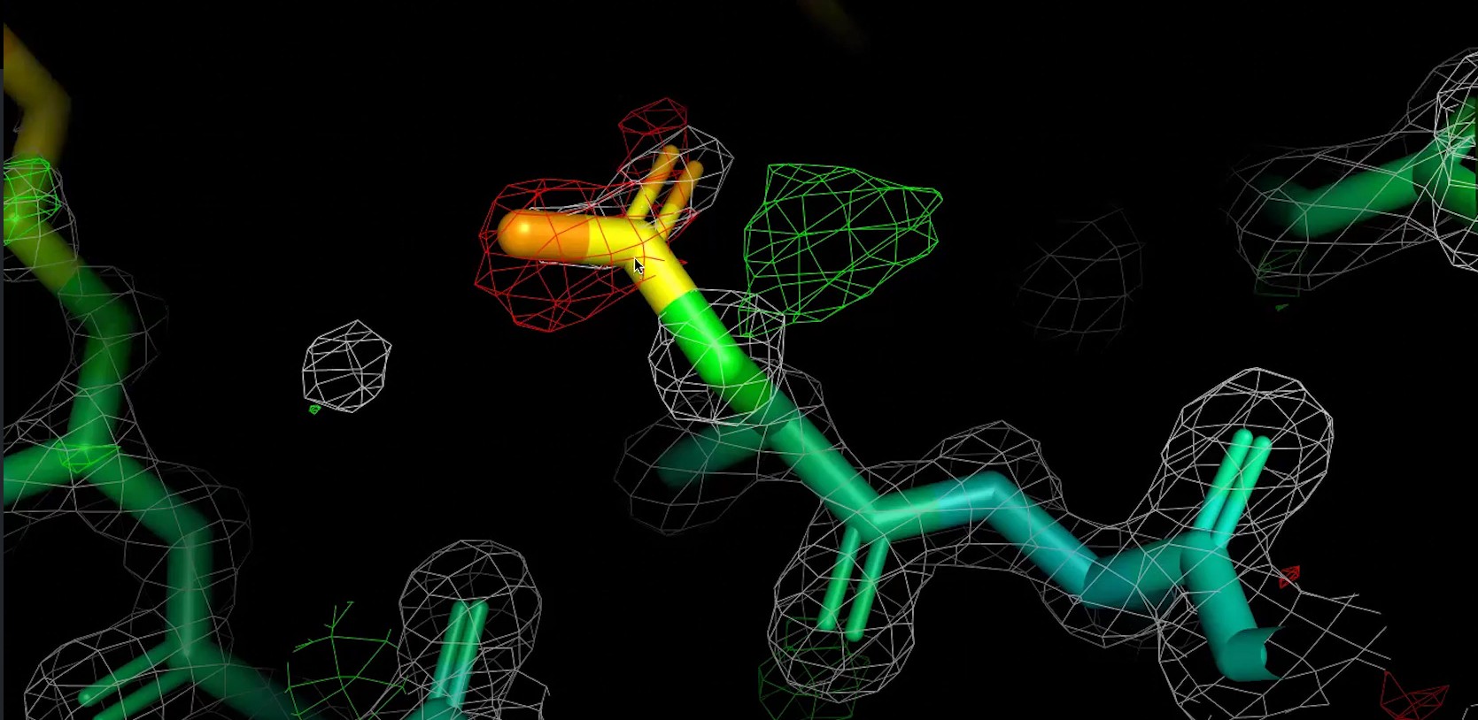
A snippet of the Fo-Fc map of 2B3P, visualised with PyMOL.

Figure 21: A snippet of the Fo-Fc map of 2B3P, visualised with PyMOL.
[By The Bumbling Biochemist, CC BY 4.0, the bumbling biochemist]

While RSCC provides a single value for a region, the Fo-Fc map offers a visual and quantitative way to identify discrepancies between the current atomic model and the experimental electron density data. It’s calculated by subtracting the electron density derived from the current model (Fc) from the electron density observed experimentally (Fo), effectively creating a map of the unexplained density.

This map highlights regions where the model either lacks density that is present experimentally or has atoms that are not supported by the data. Positive peaks, often shown as green contours, indicate observed electron density that is not accounted for by the current model, pointing to a missing atom, an unmodeled solvent molecule, or an incorrect conformation. Conversely, negative peaks, typically shown in red, signify that the model contains atoms for which there is no corresponding observed electron density, suggesting that an atom is misplaced, has too high an occupancy, or should not be there at all.

In addition to the Fo-Fc difference map, we also use a 2Fo-Fc map. This map is calculated by combining twice the observed structure factor amplitudes (2Fo) with the calculated ones (Fc), basically overlaying the difference map (Fo-Fc) onto a map that represents the model’s density (Fo). Unlike the Fo-Fc map, which only highlights errors, the 2Fo-Fc map allows us to judge how well the atoms of their model sit within the experimentally observed density. A well-refined model will show continuous 2Fo-Fc density throughout the whole structure.

Completeness

Figure 22: Visualization of missing residues in a protein structure (PDB ID: 6N1K), marked with dashed line, visualised with ChimeraX.
[By Rayhan M, CC BY 4.0]

We have established that experimental data might not always resolved every residues and atoms in our structure. Hence, crystallographer might leave those regions unmodelled, marked with a dashed line in Figure 22 (depending on the software used, sometimes it’s also represented greyed out regions). Aside from visualising the structure, you can also see the unmodelled regions on the RCSB site, as shown in Figure 23. If you want to use structure with unmodelled regions, sometimes you need to fix them. If it’s just a few atoms, especially on the sidechains, you can fix them with tools like PDBFixer. However, if it’s a whole residue, you might need to add the residue manually. We will talk about this in more detail in the next part.

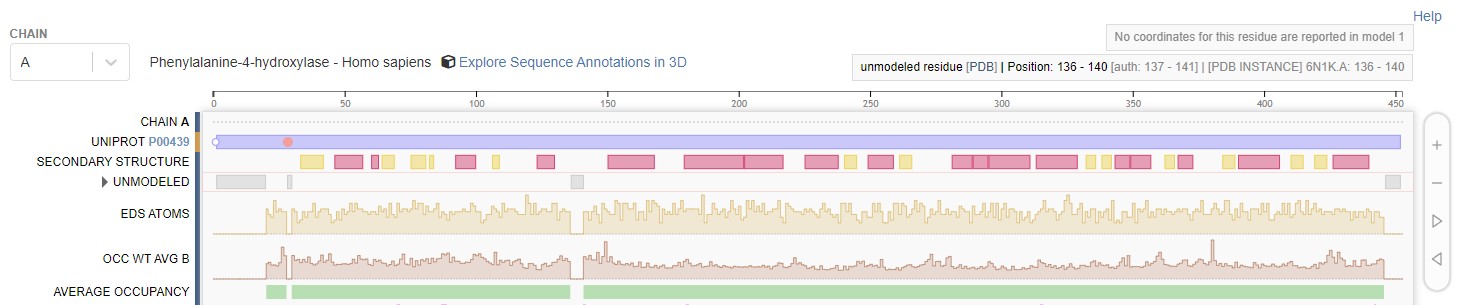
Unmodeled regions as stated on the RCSB site (PDB ID: 6N1K).

Figure 23: Unmodeled regions as stated on the RCSB site (PDB ID: 6N1K).
[By Rayhan M, CC BY 4.0]

Other metrics

The validation metrics described above are just some of the common ones. In practice, you can use many other more specific and sophisticated metrics, such as RSRZ outliers, Wilson B-Factor, EDIAm, and many more. Metric such as $R_{merge}$ which describes the agreement of individual intensities of all symmetry-equivalent reflections contributing to the same reflection, is also a good metric to use. A good set of diffraction data should have an $R_{merge}$ value < 4-5%. Signal to noise ratio, represented as $I/\sigma$ is also another important metric, ideally your signal must be higher than the background noise. Otherwise, you can’t be so sure whether what’s being captured is truly meaningful. At the end of the day, you can use whatever tool you want to assess the quality of the model you’re working with, just make sure it’s relevant to your work. RCSB has a good list of common tools which can be accessed at https://www.rcsb.org/docs/additional-resources/structure-validation-and-quality.

Storing structural data

To make our model useful and shareable, it must be stored in a standardized, machine-readable format. This is the most boring part of this post, but please bear with me. As knowing how the formats arose, their limitations, and why they still exist is a neccessity to be able to work with various programs. Please note that the snippets will display small molecules instead of proteins, as proteins are too large to be shown.

PDB

The Protein Data Bank (PDB) format is the old-timer of structural biology. Developed in the 1970s, it’s a fixed-width format with a maximum column of 80. Each line, or “record,” has a specific type (like ATOM or HETATM for non-standard residues) and data is organized into rigid columns. This format stores essential information like atom names, residue names, chain identifiers, XYZ coordinates, and the B-factors we discussed earlier.

However, its age comes with limitations. The PDB format can’t handle more than 99,999 atoms or more than 52 chains, making it unsuitable for structures like ribosomes. Moreover, it doesn’t explicitly store bond information, so visualisation software has to infer connectivity based on standard residue templates and atom distances, which can sometimes lead to errors.

HEADER    METHANE EXAMPLE
COMPND    METHANE
AUTHOR    GENERATED EXAMPLE
ATOM      1  C   ACE     1       0.000   0.000   0.000  1.00  0.00           C
ATOM      2  H1  ACE     1       0.629   0.629   0.629  1.00  0.00           H
ATOM      3  H2  ACE     1      -0.629  -0.629   0.629  1.00  0.00           H
ATOM      4  H3  ACE     1      -0.629   0.629  -0.629  1.00  0.00           H
ATOM      5  H4  ACE     1       0.629  -0.629  -0.629  1.00  0.00           H
END

mmCIF

The macromolecular Crystallographic Information File (mmCIF) is the modern, robust successor to the PDB format. It was designed specifically to overcome the limitations of its predecessor. Instead of fixed columns, mmCIF uses a flexible key-value structure, which makes it easily extensible. This format can handle structures of any size and can store a much richer set of metadata, including detailed experimental conditions and quality metrics. As of 2014, the mmCIF format is the official archival standard for the Worldwide Protein Data Bank (wwPDB), ensuring it’s the go-to format for modern structural data.

data_methane
_cell_length_a 5.0
_cell_length_b 5.0
_cell_length_c 5.0
_cell_angle_alpha 90.0
_cell_angle_beta 90.0
_cell_angle_gamma 90.0
_symmetry_space_group_name_H-M 'P 1'

loop_
_atom_site_label
_atom_site_type_symbol
_atom_site_fract_x
_atom_site_fract_y
_atom_site_fract_z
C1 C 0.0000 0.0000 0.0000
H1 H 0.1258 0.1258 0.1258
H2 H -0.1258 -0.1258 0.1258
H3 H -0.1258 0.1258 -0.1258
H4 H 0.1258 -0.1258 -0.1258

SDF

While PDB and mmCIF are designed for macromolecules, the Structure-Data File (SDF) format is the workhorse for small molecules. It’s an extension of the simpler MOL format and has a key advantage: a single SDF file can contain thousands or even millions of different molecules, making it ideal for storing chemical libraries. For each molecule, the SDF contains an atom block (with element types and 3D coordinates) and a bond block that explicitly defines which atoms are connected and the order of those bonds. Following the structural information, it can also hold associated data fields for each molecule, such as its name, chemical formula, or experimental activity.

methane
  -ISIS-  09272513222D

  5  4  0  0  0  0  0  0  0  0999 V2000
    0.0000    0.0000    0.0000 C   0  0  0  0  0  0  0  0  0  0  0  0
    0.6290    0.6290    0.6290 H   0  0  0  0  0  0  0  0  0  0  0  0
   -0.6290   -0.6290    0.6290 H   0  0  0  0  0  0  0  0  0  0  0  0
   -0.6290    0.6290   -0.6290 H   0  0  0  0  0  0  0  0  0  0  0  0
    0.6290   -0.6290   -0.6290 H   0  0  0  0  0  0  0  0  0  0  0  0
  1  2  1  0  0  0  0
  1  3  1  0  0  0  0
  1  4  1  0  0  0  0
  1  5  1  0  0  0  0
M  END
> <ID>
methane_01

> <FORMULA>
CH4

$$$$

XYZ

The XYZ format is on the simpler side of things. It does one thing and one thing only: store atomic coordinates. The format is straightforward: the first line specifies the total number of atoms, the second line is for a comment or title, and every subsequent line lists an element symbol followed by its X, Y, and Z coordinates. That’s it. It contains absolutely no information about bonds, charges, residues, or chains. This minimalist approach makes it easy to parse and is widely used in quantum chemistry programs and for simple molecular visualizations where connectivity can be easily inferred. Some programs like ORCA uses .INP which has similar structure to .XYZ.

5
Methane molecule
C     0.000000    0.000000    0.000000
H     0.629000    0.629000    0.629000
H    -0.629000   -0.629000    0.629000
H    -0.629000    0.629000   -0.629000
H     0.629000   -0.629000   -0.629000

SMILES

Unlike the previous formats, the Simplified Molecular-Input Line-Entry System (SMILES) is not a coordinate file. It is a line notation, which allows us to represent a molecule’s 2D structure as a 1D string of text. This makes it incredibly compact and perfect for database storage and searching. We can store SMILES as an .smi file.

# SMILES notation of CH4
C

Well, okay, that might not illustrate what SMILES can do, so let’s use another example: acetaminophen (N-acetyl-para-aminophenol).

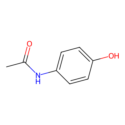
2D structure of acetaminophen, generated from the SMILES notation with RDKit.

Figure 24: 2D structure of acetaminophen, generated from the SMILES notation with RDKit.
[By Rayhan M, CC BY 4.0]

# SMILES notation of acetaminophen
CC(=O)Nc1ccc(O)cc1

While SMILES is a powerful notation, it has a quirk: different algorithms can generate different SMILES strings for the same molecule. This can make it tricky to compare molecules To solve this, “canonical SMILES” algorithms were created to assign a unique SMILES string to each molecule. There are also alternative notations, like SELFIES (Self-Referencing Embedded Strings), which are designed to always produce a valid molecule [16] .

Other formats

There are dozens of other formats that exist in the world of cheminformatics. Some notable examples would be PDBQT (used by Autodock) and PDBQR (used by PDB2PQR). Other softwares like ORCA, GROMACS, and LAMPPS also have their own formats. But need not to worry, you can convert file formats using various existing libraries (e.g., using Meeko for PDBQT or OpenBabel for general purpose conversion).

# Examples of file conversions with OpenBabel

obabel input.smi -O output.sdf --gen3d # SMILES to SDF
obabel protein.pdb -O protein.xyz # PDB to XTZ
obabel molecules.sdf -O molecules.smi # SDF to SDF
obabel input.sdf -O output.mol2 # SDF to MOL2

Some refresher on binding

At the heart of many drugs lie a fundamental biological principle: the interaction between proteins and small molecules. When proteins go awry, they often become the primary targets for therapeutic intervention.

The core idea for many drugs is quite simple: a small molecule, known as a ligand, binds to a specific site on a target protein, thereby modulating its activity. This binding can inhibit an enzyme essential for a pathogen’s survival, block a receptor to halt a pathological signal, or activate a pathway to restore normal function. Of course, there are tons of hand-waving in that explanation, but it will suffice for now. The main goal of structure-based drug design is designing ligands that are chemically and sterically complementary to a target protein’s binding site.

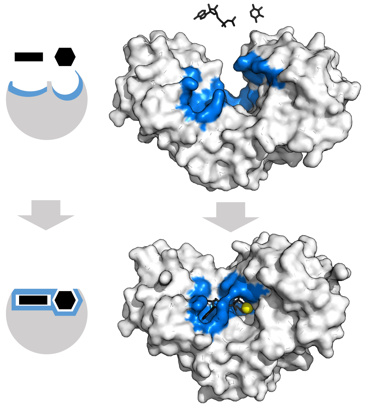
Protein can change shape by induced fit upon substrate binding to form a complex.

Figure 25: Protein can change shape by induced fit upon substrate binding to form a complex.
[By Thomas Shafee, CC BY 4.0, Wikimedia]

The induced fit model posits that the initial binding event causes conformational changes in both the protein and the ligand to achieve an optimal interaction[12]. An alternative view is the conformational seletion model. That theory suggests that proteins are dynamically changing their conformations, even without a ligand present. In that scenario, the ligand doesn’t actively change the protein’s shape, but instead “selects” and stabilises a pre-existing conformation that it can bind to. In the modern age, we see those two models as complementary, instead of mutually exclusive. A ligand may first select a favourable conformation from the protein’s existing ensemble, then followed by minor mutual adjustment via induced fit to settle the lowest energy state.

However, modelling the flexibility of a large molecule like proteins is computationally expensive, so docking programs usually use the old lock and key hypothesis instead. In that hypothesis, we model a rigid protein pocket (the lock) and a perfectly shaped ligand (the key). Yes, it’s not perfect, but when you’re trying to screen millions of potential leads, you have to make compromises. More advanced techniques like ensemble docking or flexible docking attempt to account for this inherent flexibility, but with a much higher computational cost.

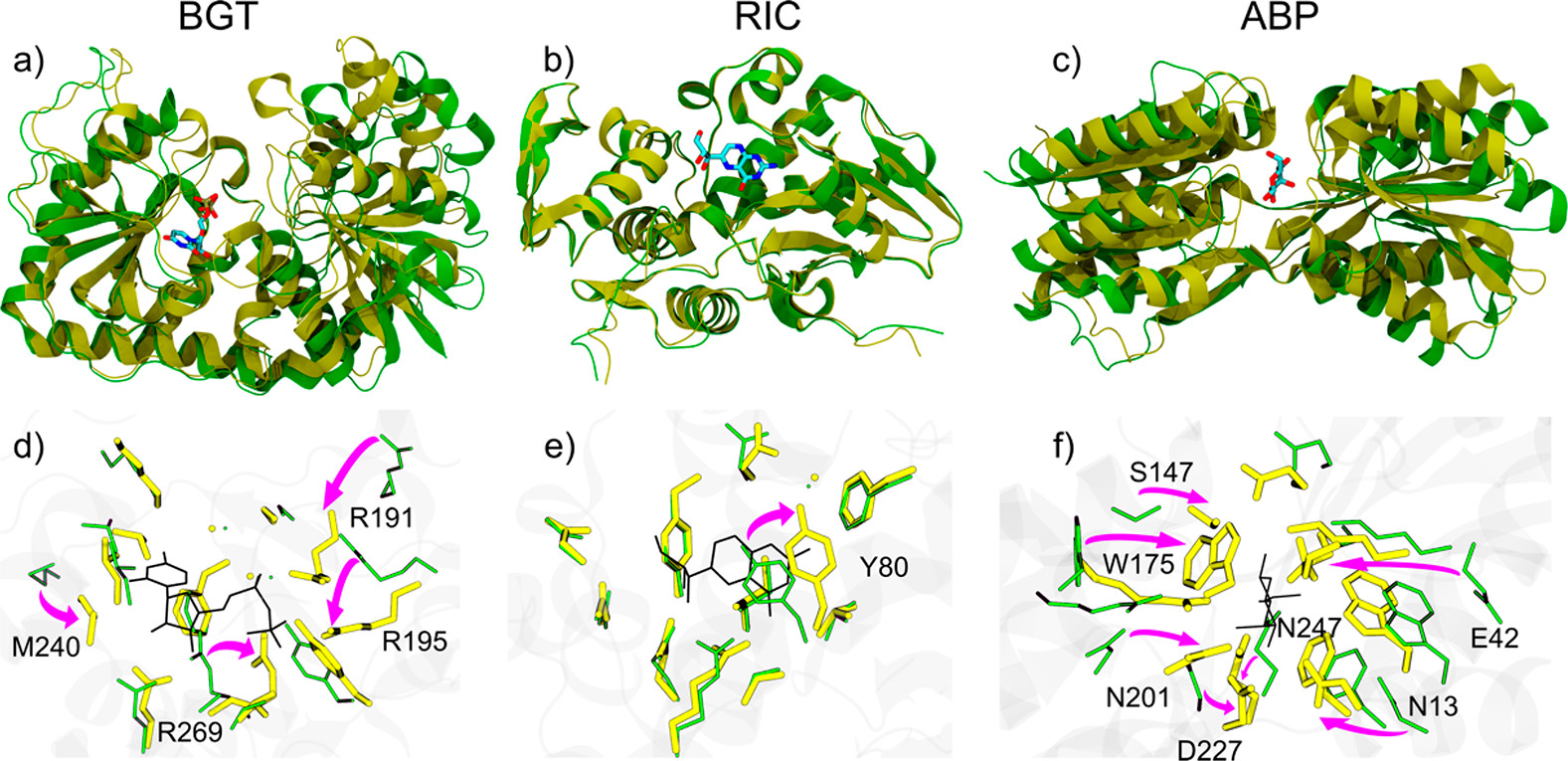
Structural changes of (a, d) BGT, (b, e) RIC, and (c, f) ABP upon binding to their respective ligands UDP, NEO, and ALL. Panels (a-c) highlight the overall conformational shifts of each protein. The apo and holo forms are shown as green and yellow ribbons, respectively. The ligands are represented as stick models coloured by atom type.

Figure 26: Structural changes of (a, d) BGT, (b, e) RIC, and (c, f) ABP upon binding to their respective ligands UDP, NEO, and ALL. Panels (a-c) highlight the overall conformational shifts of each protein. The apo and holo forms are shown as green and yellow ribbons, respectively. The ligands are represented as stick models coloured by atom type.
J. Chem. Inf. Model. 2019, 59, 4, 1515-1528.

Another very important caveat that you have to know, is that docking is usually done to the holo structure of a protein. What exactly is a holo structure? Well, you see, when a protein binds to other molecule(s), they can undergo conformational changes. In fact, when almost nothing is actively being done to them, proteins still constantly undergo conformational changes! You can see some examples of how apo and holo structures differ in the Figure 26 above.

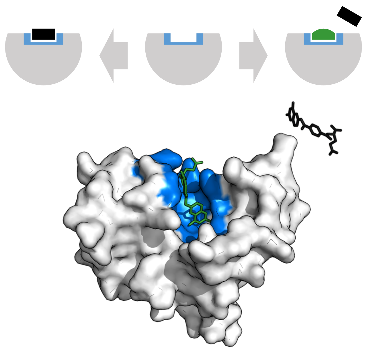
An enzyme's active site can bind a competitive inhibitor instead of its substrate, blocking access. Methotrexate inhibits dihydrofolate reductase by preventing folic acid binding. Binding site is blue, inhibitor green, substrate black (PDB: 4QI9).

Figure 27: An enzyme’s active site can bind a competitive inhibitor instead of its substrate, blocking access. Methotrexate inhibits dihydrofolate reductase by preventing folic acid binding. Binding site is blue, inhibitor green, substrate black (PDB: 4QI9).
[By Thomas Shafee, CC BY 4.0, Wikimedia]

Since docking can’t simulate proteins conformational changes, people tend to use holo structures, since they already have established binding pockets. Curious minds might wonder: “Won’t that limit our candidates to candidates that are quite similar to the native ligand?” If thought so, you’re spot on. This is a major limitation of the conventional docking approach. This inability to model protein flexibility becomes an absolute roadblock when dealing with allostery. Understanding allostery is incredibly complex, with competing theories like the Monod-Wyman-Changeux (MWC) “concerted” model, which proposes an equilibrium between two global protein states, and the Koshland-Némethy-Filmer (KNF) “sequential” model, which describes a step-wise induced fit. Because these mechanisms are fundamentally driven by large-scale, dynamic structural changes, they fall far outside the scope of rigid-protein docking. As such, the aforementioned ensemble docking, which combines MD trajectory and molecular docking to fish pockets from apo structures, is gaining traction to broaden our potential targets.

However, that’s beyond our scope here. For now, the only thing you need to know, is that usually it’s better to use the holo structures of whatever protein you’re studying, unless you absolutely know what you’re doing. Proteins’ binding pocket are usually somewhat flexible, as in, they can accept molecules that are similar enough to the native binder, as can be seen on Figure 27. That fact is what we usually try to exploit when we do virtual screening with docking programs.

Defining molecular binding

In the previous section, we have discussed about how ligands and proteins interact. However, that understanding is relatively shallow and superficial. We know they bind, but how exactly? How and why they even bind? This section will discuss just that, so that you can understand the factors affecting binding.

Measuring binding experimentally

Before going deep into the physics of binding, it’s important to understand how molecular binding is experimentally measured, as these methods provide the experimental data for validating computational predictions. Isothermal Titration Calorimetry (ITC) is widely considered the “gold standard” because it offers a complete thermodynamic profile of molecular interaction in a single, in-solution experiment. ITC directly quantifies the heat released or absorbed during molecular binding [17]. The process involves injecting small aliquots of a ligand from a computer-controlled syringe into a protein solution, maintained at a constant temperature in a sample cell. Each injection generates a heat burst; initially, a large signal indicates abundant free protein binding, which diminishes as binding sites become saturated, eventually reflecting only ligand dilution. The resulting binding isotherm allows for direct determination of binding affinity ( $K_A$ or $K_d$ ), enthalpy ( $\Delta H$ ), and stoichiometry ( $n$ ). From those metrics, the Gibbs free energy and entropy can then be calculated.

Complementing ITC, Surface Plasmon Resonance (SPR) is an optical method designed to measure binding kinetics [18]. In an SPR setup, one binding partner is immobilized on a gold-plated sensor chip. As a solution containing the other molecule flows over the surface, binding increases the mass on the chip. This mass change alters the refractive index, causing a shift in the angle of reflected polarized light, measured in Resonance Units (RU). Subsequently, a buffer without the analyte flows to measure the dissociation rate. The resulting sensorgram allows for the extraction of kinetic rate constants: the association rate constant ( $k_{on}$ or $k_A$ ) and the dissociation rate constant ( $k_{off}$ or $k_d$ ). In the modern drug design paradigm, SPR is particularly useful thanks to its capability of measuring binding kinetics, hence allowing us to study the residence time[19] of our ligands.

Binding thermodynamics

Consider binding as an equilibrium of a protein $P$ and a ligand $L$ in an aqueous box of volume V at temperature T, which can be stated as

P + L \rightleftharpoons PL

At equilibrium, the ratio of the binding ( $k_{on}$ ) and unbinding ( $k_{off}$ ) rate constants defines the equilibrium association constant, $K_A$ :

K_A = \frac{k_{\text{on}}}{k_{\text{off}}} = \frac{[PL]}{[P][L]} = \frac{1}{K_d}

Following that, we can define the molar-standard Gibbs free energy of binding as

\Delta G_{bind} = RTlnK_d = -RTlnK_A

where $K_A$ is the association constant, $K_d$ the dissociation constant, $R$ the gas constant, and $T$ the temperature in kelvin. We can further decompose it into its constituent parts:

\Delta G_{bind} = \Delta H - T\Delta S

In computational models, this is often approximated by separating terms for the molecules in a vacuum, the effect of the solvent (water), and the loss of molecular freedom: $\Delta G_{bind} \approx \Delta E_{gas} + \Delta G_{solv} - T\Delta S_{conf}$ Here, $\Delta E_{gas}$ is the change in interaction energy in a vacuum, $\Delta G_{solv}$ is the free energy change of solvation, and $\Delta S_{conf}$ is the change in configurational entropy. Let’s break down what these mean.

The enthalpy change ( $\Delta H$ ) is about the energy of connections and forces. It’s largely captured by the vacuum interaction term ( $\Delta E_{gas}$ ) and the enthalpic part of solvation. The entropy change ( $\Delta S$ ) is about the change in disorder or “freedom” in the system. It includes the configurational entropy of the molecules ( $\Delta S_{conf}$ ) and the entropy of the surrounding solvent.

The Entropy Term

Let’s start with entropy. Binding is an act of ordering. Before binding, the protein and ligand can move, rotate, and tumble freely in solution. When they form a complex, they lose most of this translational and rotational freedom. Furthermore, flexible parts of the ligand (rotatable bonds) become locked into a specific conformation. This loss of freedom is a significant decrease in configurational entropy ( $\Delta S_{conf}$ is negative), which makes the $-T\Delta S_{conf}$ term positive and thus unfavorable for binding.

The Enthalpy Term

Enthalpy is primarily about the energetic interactions formed and broken during binding. In a computational model, we first consider the interaction energy in a vacuum ( $\Delta E_{gas}$ ), which is the sum of several forces:

\Delta E_{gas} = \Delta E_{vdw} + \Delta E_{coul} + \Delta E_{internal}

The internal energy ( $\Delta E_{internal} = \Delta E_{bond} + \Delta E_{angle} + \Delta E_{dihed}$ ) represents the strain a molecule might adopt to fit into a binding site. To fit optimally, a ligand might have to stretch its bonds or twist into a less-than-ideal shape, which carries an energy penalty. A good ligand fits comfortably without too much strain. In many calculations, this term is assumed to be small and is often ignored. The key drivers are the non-bonded interactions.

Van der Waals interaction

$E_{vdw}$ or van der Waals is a broad range of interactions: ranging from London dispersion, dipole-dipole, and induced-dipole. Without going into the nitty gritty part, what you have to know is that van der Waals interactions are caused by the movement of electrons. Quantum mechanics posits that the energy of electrons are never zero, that is that they constantly move in an atom through the Schrodinger equation and the Heisenberg uncertainty principle. Hence, at any time, the charge of an atom can be distributed in a different manner. Sometimes electrons are distributed asymmetrically, creating two poles—dipoles—that is one side will be more positive/negative than the other. Usually, many programs will calculate vdW using the Lennard-Jones (LJ) equation:

V_{LJ}(r) = 4\epsilon \left[ \left( \frac{\sigma}{r} \right)^{12} - \left( \frac{\sigma}{r} \right)^6 \right]

Keep in mind that LJ is an approximation, same goes with Morse potential, or any other equations. However, LJ is good enough for most use cases. A negative value means an attraction, while a positive value signifies a repulsion. We can see that there are several parameters in that equations, $\epsilon$ represents the “depth” of the potential well, that is the maximum strength of the attraction between the two particles. $\sigma$ represents the finite distance at which the potential energy is zero. It can be thought of as the effective “size” of a particle or the collision diameter. Lastly, $r$ is the distance between centre of the two particles.

If we take a closer look, we can divide divide the equation into two parts: the repulsive terms $\left( \frac{\sigma}{r} \right)^{12}$ and the attraction terms $\left( \frac{\sigma}{r} \right)^{6}$ . Since the repulsive term has a bigger exponent $(^{12})$ , it will grow much faster than the attraction terms, this means our vdW energy will quickly become repulsive as molecules get too close, and rapidly approach zero as they move further apart. Moreover, if the distance is shorter than the effective size ( $\sigma$ ), the equation will even produce a positive number, indicating that the particles are too close and repelling each other. I recommend watching this video below by NucleusBiology.

Electrostatic interaction

Now, let’s continue with the other term: $E_{coul}$ . This term basically quantify the effect of electrostatic interaction, which is governed by the Coulomb’s law:

U = k\frac{q_1q_2}{r}

with $k = 1/4\pi\varepsilon_0$ in a vacuum, $q_1q_2$ the partial charge of the particles, and $r$ the distance between the particles. The value of $\varepsilon_0$ is approximately $\varepsilon_0 = 8.8541878128\times10^{-12}\ \mathrm{F\,m^{-1}}$ . If we plug in some numbers, you will notice that the energy produced by this term is massive. Let’s try calculate an example with a distance of $3 \AA$ , $q_1$ of $1.602 \times 10^{-19} C$ , and $q_2$ of $-1.602 \times 10^{-19} C$ .

U = \frac{1}{4\times\pi\times8.8541878128\times10^{-12}}\frac{1.602 \times 10^{-19} \times -1.602 \times 10^{-19}}{3 \times 10^{-10}} = -7.68 \times 10^{-19} J \approx -110.7\ kcal/mol

Whoops! That’s not realistic at all, right? And that’s just between two pair of atoms. The reason for this discrepancy is that our calculation was for a vacuum. In a biological system, everything is surrounded by a solvent (usually water in biological systems). The powerful influence of water is captured in the $G_solv$ term, which is arguably the most complex and important factor in molecular binding. We can break it down into two main physical phenomena:

G_{solv} = G_{polar\_solv} + G_{hydrophobic}

Polar solvation and desolvation penalty

Before binding, any polar or charged groups on both the ligand and the protein’s binding pocket are happily interacting with water. Because water is a polar molecule, it forms stable, ordered “hydration shells” around these charged surfaces.

llustration of the desolvation penalty.

Figure 28: Illustration of the desolvation penalty.
[Courtesy of Francesca Peccati and Gonzalo Jiménez-Osés, Enthalpy-Entropy Compensation in Biomolecular Recognition: A Computational Perspective, ACS Omega 2021 6 (17), 11122-11130, DOI: 10.1021/acsomega.1c00485]

When the ligand enters the binding pocket, these organized water molecules must be pushed out of the way. This has an energy cost, known as the desolvation penalty, because we have to break the favorable hydrogen bonds between water and the solute molecules. For the binding to be favorable, the new hydrogen bonds and electrostatic interactions formed between the protein and the ligand must be strong enough to overcome this penalty.

The hydrophobic effect

The second, and often dominant, part of solvation is the hydrophobic effect. You might recall back in elementary school that water and oil don’t mix due to different density. Well, that’s just plain wrong. Density does make oil floats, but it’s not what makes them don’t mix. Luckily, by high school, most people learn the concept of polarity and the explanation shifted to: they don’t mix because water is polar, while oil is nonpolar. But, even that explanation is incomplete. Hydrophobicity is not due to nonpolar molecules repelling water; it’s driven by the entropy of the surrounding water molecules.

Water, as a polar molecule, forms a dynamic network of hydrogen bonds. When these bonds form, energy is released, so the overall system’s enthalpy is lowered, making it more stable. These bonds are transient, meaning water molecules can change partners freely. This freedom of movement contributes to the high entropy of bulk water.

When you introduce nonpolar molecules to water, they cannot form hydrogen bonds. To maximize the hydrogen bonding within the water network, the water molecules are forced to arrange themselves into ordered, cage-like structures around the nonpolar solutes. This high degree of order restricts the water molecules’ freedom of movement, causing a large decrease in the solvent’s entropy, which is thermodynamically unfavorable. To minimize this unfavorable entropy cost, the system pushes the nonpolar molecules together. This aggregation reduces the total surface area that needs to be ‘caged,’ liberating the ordered water molecules back into the free-moving bulk solvent. This release of water molecules results in a significant increase in the overall entropy of the system, which is the primary driving force of the hydrophobic effect.

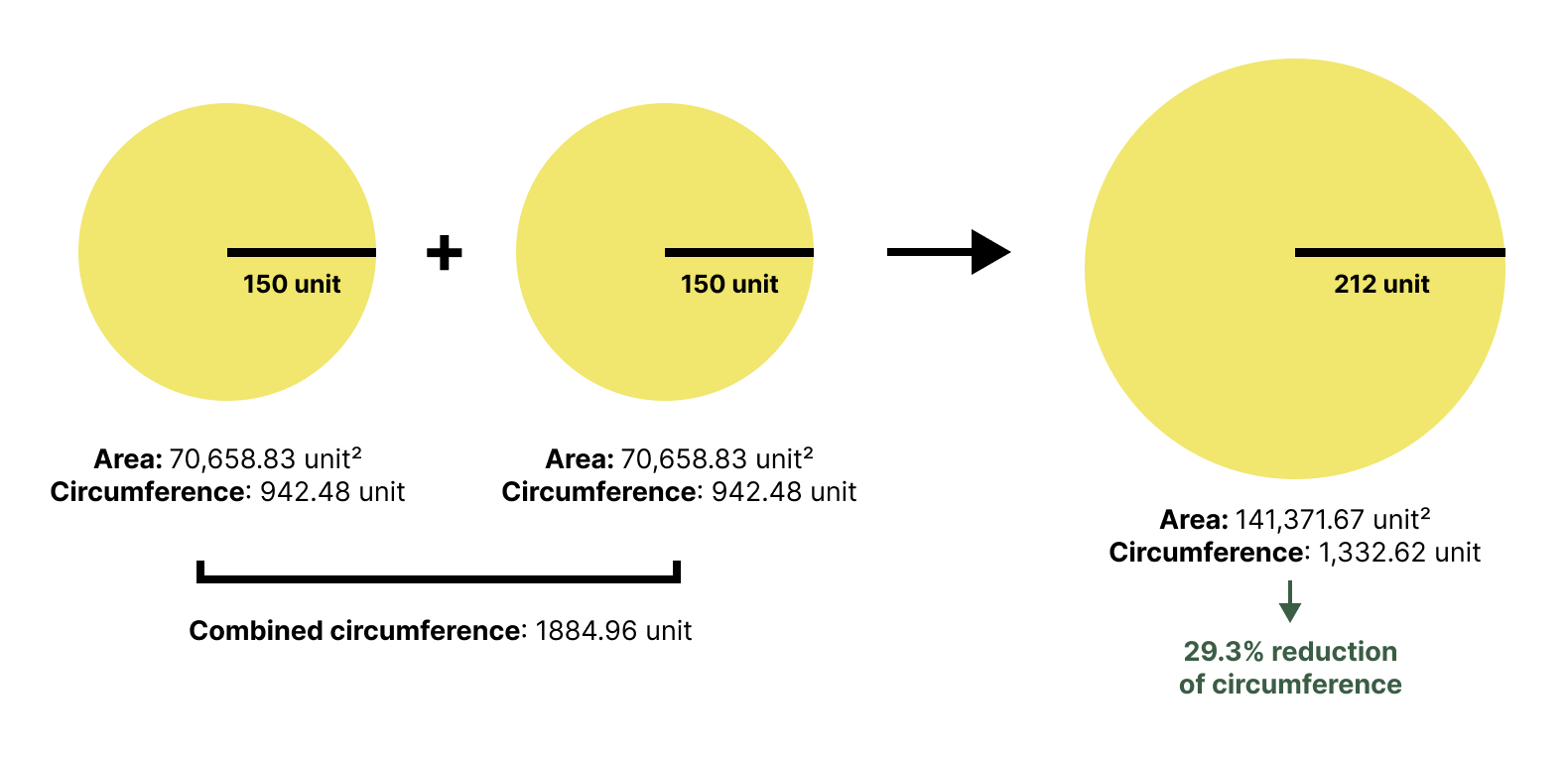
Merging two circles into one circle reduces the total surface area, illustrating the principle behind hydrophobic aggregation.

Figure 29: Merging two circles into one circle reduces the total surface area, illustrating the principle behind hydrophobic aggregation.
[By Rayhan M, CC BY 4.0]

So, as you can see, hydrophobicity is mainly driven by water as the solvent. This effect applies in the context of protein-ligand binding too. Proteins consist of various residues, some are polar, some are nonpolar. The same goes with a ligand; it can have both polar and nonpolar parts. To maximize the entropy of the system, water will “push” the nonpolar part of the ligand and the nonpolar residues of the protein’s pocket together, minimizing the contact of water with those nonpolar regions.

To recap, interactions mediated by water are complex. On one hand, water can help our ligand bind by “pushing” the nonpolar side of our ligand to the hydrophobic residue on the pocket. However, in the process, that event might also disrupt the preexisting hydration shells formed by water and hydrophilic residues on the pocket. This dynamic is subject to studies when designing the hydrophobicity and hydrophilicity of a ligand.

Those solvent-related phenomenons also explain why water is so good at screening electrostatic interactions. The hydration shell effectively places a cloud of opposite partial charges around an ion, weakening its interaction with other ions. It is important to note that the water molecules don’t bind to the ions, they reduce the interaction strength, hence the term screening. For example, if you have an $Na^+$ ion, the positive charge will be screened by the more negative side of the water molecules (oxygen-side). The opposite is true for Cl- and the more positive side of the water molecules (hydrogen-side). This screening ability can be quantified by the dielectric constant ( $\varepsilon_r$ ). Water has a high dielectric constant of ~80, meaning it reduces the electrostatic force to about 1/80th of its strength in a vacuum. This is why adding $\varepsilon_r$ to the Coulomb’s law equation gives a much more realistic energy value:

U = \frac{1}{4\pi\varepsilon_0\varepsilon_r} \frac{q_1q_2}{r}

If we redo our initial calculation with the $\varepsilon_r$ set to 78.5, our $E_{coul}$ becomes -1.41 kcal/mol, a much more sensible number! When water is excluded from the binding pocket, the local environment becomes nonpolar (like oil), with a very low dielectric constant ( $\varepsilon_r \approx 4$ ). In this environment, the direct electrostatic attractions that do form between the ligand and protein are much stronger. Keep in mind that the dialectric constant is not homogenous everywhere, for example the inner protein pocket can have fewer water molecules, making their screening power way lower.

While simple models like a distance-dependent dielectric can approximate these complex effects, more sophisticated methods are needed for higher accuracy, leading to two primary strategies: explicit and implicit solvation. Explicit solvation is the most physically intuitive and accurate approach. It involves building a simulation box where the protein and ligand are surrounded by thousands of individual, explicitly defined water molecules. This method, typically used in molecular dynamics (MD), can capture specific, directed interactions like water-mediated hydrogen bonds.

However, modelling the movement of every single water molecule is computationally expensive. For this reason, molecular docking often rely on implicit solvation models. Instead of simulating individual water molecules, it treats the solvent as a continuous, uniform medium with a single dielectric constant. Other methods like the Poisson-Boltzmann (PB) equation or analytical approximations like the Generalized Born (GB) model can used to calculate the electrostatic contribution of this continuum. While less accurate than explicit models, implicit solvation provides a good-enough approximation of solvent effects at a fraction of the computational cost. We won’t talk too much about the math, but it’s important to know that solvation effects, for the most part are heavily simplified in in silico methods due to computational constraints.

Striking the balance

Entropy and enthalpy cancels out.

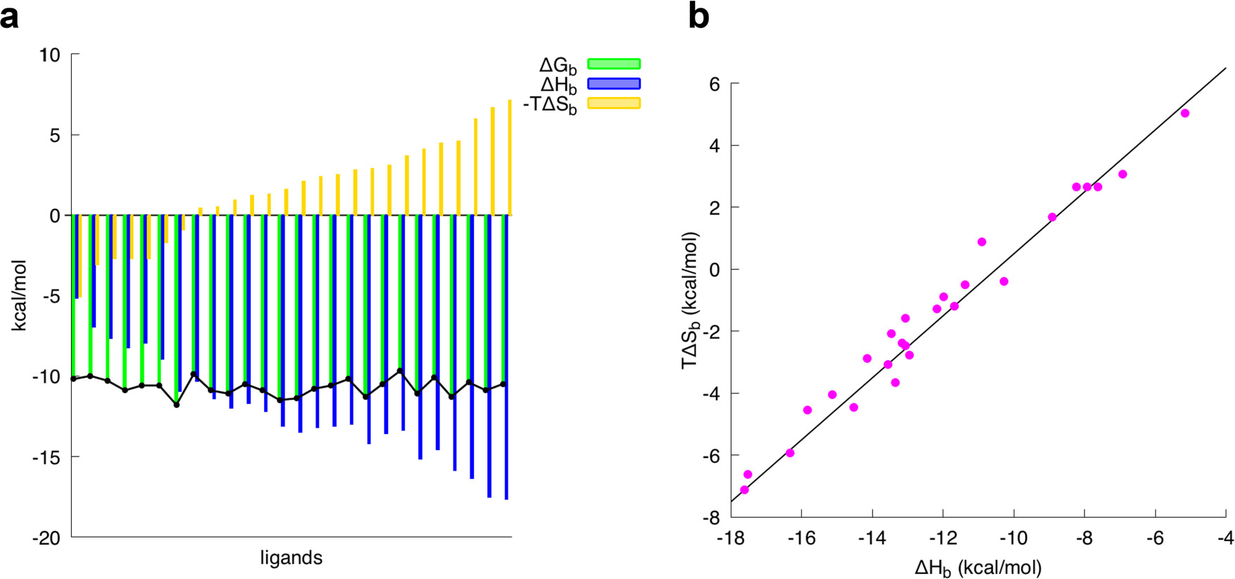
Figure 30: Entropy and enthalpy cancels out.
[Courtesy of Francesca Peccati and Gonzalo Jiménez-Osés, Enthalpy-Entropy Compensation in Biomolecular Recognition: A Computational Perspective, ACS Omega 2021 6 (17), 11122-11130, DOI: 10.1021/acsomega.1c00485]

We have talked about both enthalpy and entropy, and how they can be used to calculate the binding affinity of a molecule. However, in reality, the binding affinity is a complex interplay of both. For example, in Figure 30, we can see that the entropy and enthalpy cancels out, any gain in enthalpy is offset by the loss in entropy. As our enthalpy get more favourable, the entropy get less favourable, making the overall binding affinity remain constant. This phenomenon is known as enthalpy-entropy compensation [20].

To give you a better idea, let’s take a look at the binding affinity of a molecule. Let’s say we have a complex with a binding affinity of -10 kcal/mol. If we try to refine our ligand by adding a new site for hydrogen bonding, we can perhaps decrease the Gibbs free energy by 1 kcal/mol. However, this hydrogen bond also reduces the entropy of the system by 1 kcal/mol, since any previously free rotamer is now locked in a specific, rigid conformation. As a result, the overall binding affinity remains roughly the same, or sometimes even become less favourable. Due to this phenomenon, it’s important to not only consider the enthalpy of the binding, but also the entropy.

Conclusion

This part of our journey has finally come to an end. This is the longest article I have ever written, taking me several weeks to complete. I hope that by learning about the intricate processes of protein structure determination, you have gained a new appreciation for the complexities of the field. Furthermore, I hope this post serves as a useful guide for those learning molecular docking, as it is very easy to be misled by a bogus result without the proper foundational knowledge. We have also covered the major interactions in protein-ligand binding, which we will explore further in the next installment from a computational perspective.

I hope you enjoyed reading this article, or at the very least, found it helpful. See you in the next one.

A Primer on Molecular Docking (Part 1): Structure & Binding

References

GENERAL REFERENCES
[1] Rupp, B. (2009). Biomolecular Crystallography: Principles, Practice, and Application to Structural Biology. Garland Science. ↩
[2] Rhodes, G. (2006). Crystallography made crystal clear: A Guide for Users of Macromolecular Models. Academic Press. ↩
[3] McPherson, A. (2011). Introduction to macromolecular crystallography. John Wiley & Sons. ↩
[4] Wlodawer, A., Minor, W., Dauter, Z., & Jaskolski, M. (2007). Protein crystallography for non-crystallographers, or how to get the best (but not more) from published macromolecular structures. FEBS Journal, 275(1), 1-21. https://doi.org/10.1111/j.1742-4658.2007.06178.x ↩
[5] Du, X., Li, Y., Xia, Y., Ai, S., Liang, J., Sang, P., Ji, X., & Liu, S. (2016). Insights into Protein–Ligand Interactions: Mechanisms, Models, and Methods. International Journal of Molecular Sciences, 17(2), 144. https://doi.org/10.3390/ijms17020144 ↩
REFERENCES FOR SPECIFIC TOPICS
[6] Based on data from https://www.rcsb.org/stats/summary. ↩
[7] Dyda, F., Hickman, A. B., Jenkins, T. M., Engelman, A., Craigie, R., & Davies, D. R. (1994). Crystal structure of the catalytic domain of HIV-1 integrase: similarity to other polynucleotidyl transferases. Science (New York, N.Y.), 266(5193), 1981-1986. https://doi.org/10.1126/science.7801124 ↩
[8] Bujacz, G., Jaskólski, M., Alexandratos, J., Wlodawer, A., Merkel, G., Katz, R. A., & Skalka, A. M. (1995). High-resolution structure of the catalytic domain of avian sarcoma virus integrase. Journal of molecular biology, 253(2), 333-346. https://doi.org/10.1006/jmbi.1995.0556 ↩
[9] Bujacz, G., Jaskólski, M., Alexandratos, J., Wlodawer, A., Merkel, G., Katz, R. A., & Skalka, A. M. (1996). The catalytic domain of avian sarcoma virus integrase: conformation of the active-site residues in the presence of divalent cations. Structure (London, England : 1993), 4(1), 89-96. https://doi.org/10.1016/s0969-2126(96)00012-3 ↩
[10] Maignan, S., Guilloteau, J. P., Zhou-Liu, Q., Clément-Mella, C., & Mikol, V. (1998). Crystal structures of the catalytic domain of HIV-1 integrase free and complexed with its metal cofactor: high level of similarity of the active site with other viral integrases. Journal of molecular biology, 282(2), 359–368. https://doi.org/10.1006/jmbi.1998.2002 ↩
[11] Goldgur, Y., Dyda, F., Hickman, A. B., Jenkins, T. M., Craigie, R., & Davies, D. R. (1998). Three new structures of the core domain of HIV-1 integrase: an active site that binds magnesium. Proceedings of the National Academy of Sciences of the United States of America, 95(16), 9150-9154. https://doi.org/10.1073/pnas.95.16.9150 ↩
[12] Takaba, K., Maki-Yonekura, S., Inoue, I., Tono, K., Hamaguchi, T., Kawakami, K., Naitow, H., Ishikawa, T., Yabashi, M., & Yonekura, K. (2023). Structural resolution of a small organic molecule by serial X-ray free-electron laser and electron crystallography. Nature Chemistry, 15(4), 491-497. https://doi.org/10.1038/s41557-023-01162-9 ↩
[13] Lu, H., & Tonge, P. J. (2010). Drug-target residence time: critical information for lead optimization. Current opinion in chemical biology, 14(4), 467-474. https://doi.org/10.1016/j.cbpa.2010.06.176 ↩
[14] Søndergaard, C. R., Olsson, M. H. M., Rostkowski, M., & Jensen, J. H. (2011). Improved treatment of ligands and coupling effects in empirical calculation and rationalization of PKA values. Journal of Chemical Theory and Computation, 7(7), 2284-2295. https://doi.org/10.1021/ct200133y ↩
[15] Olsson, M. H. M., Søndergaard, C. R., Rostkowski, M., & Jensen, J. H. (2011). PROPKA3: Consistent treatment of internal and surface residues in Empirical PKAPredictions. Journal of Chemical Theory and Computation, 7(2), 525-537. https://doi.org/10.1021/ct100578z ↩
[16] Krenn, M., Häse, F., Nigam, A., Friederich, P., & Aspuru-Guzik, A. (2020). Self-referencing embedded strings (SELFIES): A 100% robust molecular string representation. Machine Learning Science and Technology, 1(4), 045024. https://doi.org/10.1088/2632-2153/aba947 ↩
[17] Saponaro A. (2018). Isothermal Titration Calorimetry: A Biophysical Method to Characterize the Interaction between Label-free Biomolecules in Solution. Bio-protocol, 8(15), e2957. https://doi.org/10.21769/BioProtoc.2957 ↩
[18] Sparks, R. P., Jenkins, J. L., & Fratti, R. (2019). Use of Surface Plasmon Resonance (SPR) to Determine Binding Affinities and Kinetic Parameters Between Components Important in Fusion Machinery. Methods in molecular biology (Clifton, N.J.), 1860, 199-210. https://doi.org/10.1007/978-1-4939-8760-3_12 ↩
[19] Lu, H., & Tonge, P. J. (2010). Drug-target residence time: critical information for lead optimization. Current opinion in chemical biology, 14(4), 467-474. https://doi.org/10.1016/j.cbpa.2010.06.176 ↩
[20] Peccati, F., & Jiménez-Osés, G. (2021). Enthalpy-Entropy compensation in Biomolecular Recognition: a Computational perspective. ACS Omega, 6(17), 11122-11130. https://doi.org/10.1021/acsomega.1c00485 ↩
Disclaimer
While every effort has been made to ensure the accuracy of this article, it is not intended as a substitute for rigorous academic research. I make no guarantee that the content is error-free. I highly encourage readers to corroborate the information presented here with primary sources.
Acknowledgments
I would like to thank the structural biology community for making structural data freely available, enabling research and education worldwide. Hopefully, this article can serve as a good starting point for those who are interested in learning about molecular docking.
Author Contributions
This article was compiled from various sources by the author. All figures were created or adapted with appropriate attribution to their original sources.
License
Figures and text are licensed under Creative Commons Attribution CC-BY 4.0 with the source available on GitHub, unless noted otherwise.